I tried replacing cloud AI with local models. The useful result was a hybrid workflow.
TL;DR
- I spent three weeks, July 9–31, 2026, doing all my coding work with local models only, then switched cloud models back on and kept measuring.
- Local 27B-class models such as Qwen 3.8 27B handled a large share of daily work: repo search, unit tests, bug spotting, and implementing small to medium features from a clear spec.
- They fell short on long refactors, large repositories, and questions that need broad knowledge rather than reasoning, such as Terraform on Azure.
- Once I could use cloud models again, a clear split appeared: cloud calls had a median of about 92k input tokens, local calls about 31k.
- What stayed is a hybrid, spec-driven workflow: cloud models design, plan and review, local models implement. The orchestrator agent behind it is available to download.
The bet
About half a year ago, when I started exploring the idea of hosting Foundational models myself, an interesting dicussion popped up at work about the emerging "Token Economy". This new world where companies were (and are still) spending staggering amounts of money on AI usage through the ever so etherial AI credit system. With my newfound hobby for local AI, I was wondering what place it could have in the Token Economy.
So, in July 2026 I switched off cloud AI for my day-to-day software engineering work. The hypothesis was simple and purposefully naive:
For the work I actually do, a sufficiently capable model running on my own hardware could replace cloud AI for most tasks without materially reducing my productivity.
Or, as a Dutch person, I was wondering: could I replace my Ferrari with a bicycle?
I did not expect a clean yes or no, but I did expect the answer to be about replacement. It turned out to be about something else. Local models earned a permanent place in how I work, and cloud models kept theirs. What changed was that I stopped thinking of them as competitors and started routing work between them. I hypothesized replacement; I found complementarity.
This post is a field report rather than a benchmark. I measured what I could with the telemetry my editor already produces, and I describe the rest as my own experience on my own hardware. Where the data can say something, I show it. Where it cannot, I say so.
Three weeks without cloud AI
The experiment ran from July 9 to July 31, 2026 with myself as guinea pig. During those three weeks I did all of my regular work with on-device models only: no frontier model in the editor, no chat assistant in the browser, no quiet exceptions. Before the experiment started I had already turned on the OpenTelemetry export in GitHub Copilot, so every model call, tool call and agent turn from my editor was recorded.1 On August 1 I switched cloud models back on, and the hybrid period that followed is the second half of the data.
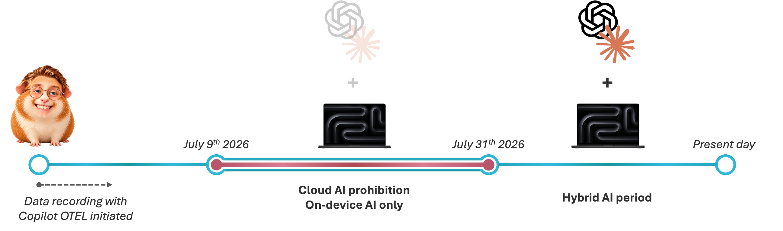
Three weeks is long enough to stop treating the setup as a novelty. By the second week the question was no longer whether a local model could answer a prompt, but whether I could get through a normal working day with it. That is a much harder and more honest test.
Running a model means running a stack
The first thing I learned is that "running a local model" is not a single decision. It is a stack of decisions which effectively need to be taken in parallel, and every layer can make or break the experience.
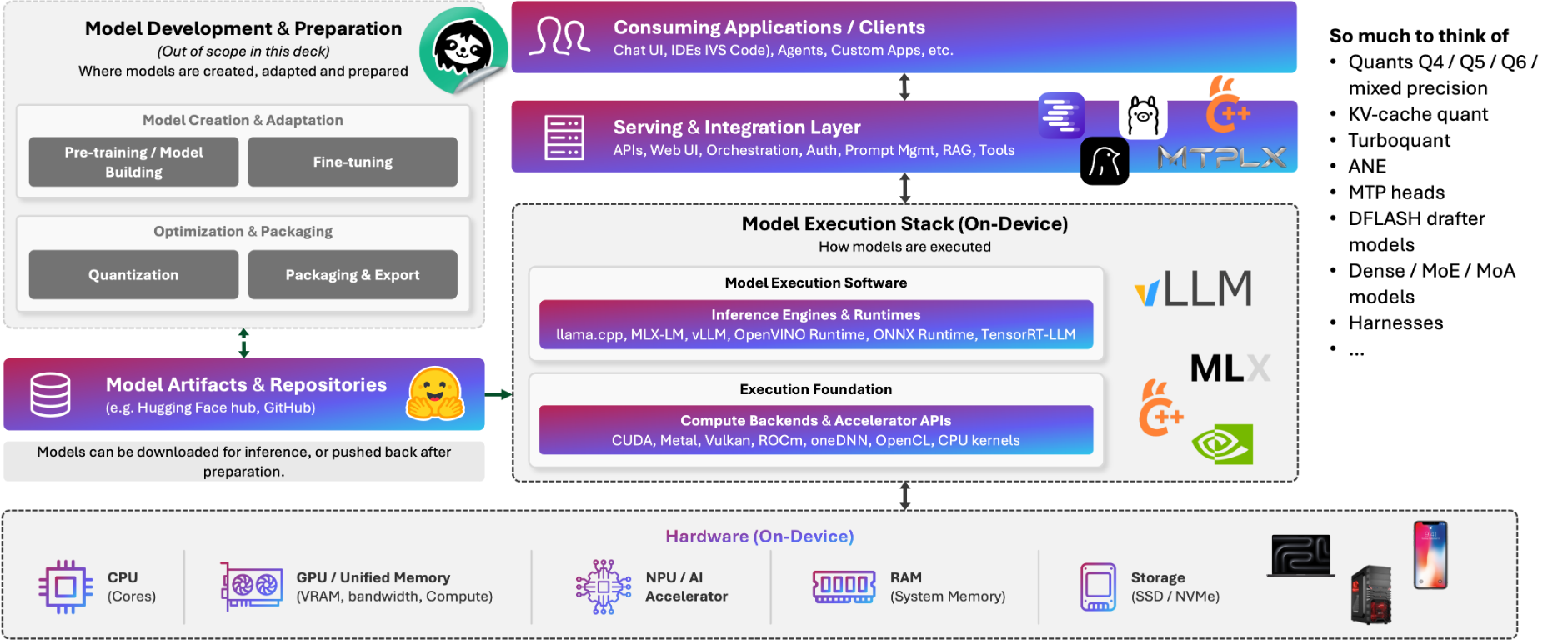
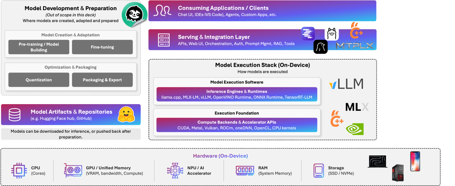
See below diagram of my first interpretation of the local AI stack. If the diagram feels somewhat overwhelming, excellent, that is deliberate. When I presented it to my colleagues, my intention was precisely that: quantization, KV-cache management, tensor parallelism, continuous batching, prefill and decode throughput, P99 latency, speculative decoding, MTP heads, mixture-of-experts, inference runtimes, and agent harnesses. You do not need to know what any of these mean.
That flood of options, settings and acronyms is exactly what going down the local AI rabbit hole feels like. The broader point I am making here, is that hosting foundational models should be treated as an engineering discipline of its own right, with its own architectural decisions, performance trade-offs, and operational challenges.
I ran the experiment on two machines: my company MacBook Pro and a home-built Ubuntu desktop server with two consumer GPUs on a much older platform.
| MacBook Pro (work laptop) | Desktop PC (home-built) | |
|---|---|---|
| Form factor | 16-inch laptop | Tower |
| OS | macOS | Ubuntu |
| Chip / CPU | Apple M5 Max | Intel Core i5-4690K |
| GPU | Integrated M5 Max GPU | 2× NVIDIA RTX 3060 (12 GB each) |
| Memory for models | 64 GB unified memory | 24 GB VRAM (2 × 12 GB) |
| System RAM | Shared with the GPU (same 64 GB) | 32 GB DDR3 |
| Motherboard | n/a | MSI Z97S Krait |
| Power supply | Built-in | 850 W |
| Main runtime | LM Studio | llama.cpp (llama-server, CUDA build) |
| Other runtimes used | MTPLX, oMLX, DFlash | n/a |
On the Mac I mostly serve models through LM Studio. Along the way I tried a long list of other runtimes and inference engines, including DFlash, oMLX and MTPLX. Today, LM Studio with the Splash engine is by far the best overall option for Qwen 3.8 27B on that machine. On the desktop I run llama.cpp directly. The main model there is a Q4 quantization of the same Qwen 3.8 27B, split across both GPUs with tensor split, with multi-token prediction turned on, some kernel customization, and a community "GPU unlocker" project that removes the cap NVIDIA sets by default on tensor cores for FP16 / BF16 /TF32 operations of their consumer grade graphics cards.
Show the llama.cpp server command for the dual RTX 3060 desktop
After a lot of tuning, this is the command I run Qwen 3.8 27B with on the two RTX 3060 cards:
GGML_CUDA_DISABLE_GRAPHS=1 \
~/qwen38-27b-rtx3060-dcfr/third_party/llama.cpp/build-cuda/bin/llama-server \
  -m ~/qwen38-27b-rtx3060-dcfr/models/q4/Qwen3.8-27B-UD-Q4_K_XL.gguf \
  -ngl all \
  -sm tensor \
  -ts 1,1 \
  -c 128000 \
  -fa on \
  -ctk q8_0 \
  -ctv q8_0 \
  -b 256 \
  -ub 64 \
  --spec-type draft-mtp \
  --spec-draft-n-max 2 \
  --spec-draft-ngl all \
  --spec-draft-type-k q4_0 \
  --spec-draft-type-v q4_0 \
  --context-shift \
  --keep 4096 \
  --parallel 1 \
  --cache-prompt \
  --cache-reuse 256 \
  --host 0.0.0.0 \
  --port 11434 \
  --timeout 1800 \
  --metrics
What the important settings do:
-ngl all -sm tensor -ts 1,1: puts every layer on the GPUs and splits the tensors evenly across both cards.-c 128000: a 128K-token context window.-fa on -ctk q8_0 -ctv q8_0: flash attention plus an 8-bit KV cache, which is what makes a 128K context fit in 24 GB of VRAM.-b 256 -ub 64: smaller logical and physical batch sizes, which leave VRAM free for the context.--spec-type draft-mtp --spec-draft-n-max 2: speculative decoding with the model's own multi-token prediction heads, drafting up to two tokens at a time. The drafter's KV cache runs at 4-bit (q4_0).--context-shift --keep 4096: when the context fills up, older tokens are dropped but the first 4,096 (the system prompt and instructions) are kept.--cache-prompt --cache-reuse 256: reuses the KV cache across requests, so an agent sending the same long prefix again does not pay to process it twice.--parallel 1: one request slot, so the whole context belongs to a single agent.--host 0.0.0.0 --port 11434 --timeout 1800 --metrics: serves on the local network, with a 30-minute timeout for long agent turns and a Prometheus metrics endpoint.GGML_CUDA_DISABLE_GRAPHS=1: turns off CUDA graphs. This was more stable with this setup.
The kernel customization and the GPU unlocker mentioned above are not part of this command. They live in the build and in the driver setup.
None of that is plug-and-play. Quantization level, KV-cache settings, context length, drafter models and the runtime itself all moved the result, sometimes by a lot. A model that felt unusable with one configuration was perfectly fine with another. That is the hidden cost of local AI: you are not just choosing a model, you are operating AI infrastructure.
The model-size sweet spot
The second lesson was about size. Smaller models are fast and cheap to run, but below a certain size they stop being useful for agentic coding work. Larger models do not fit comfortably on the hardware I have. In between there is a class of models that, for me, hits the sweet spot.
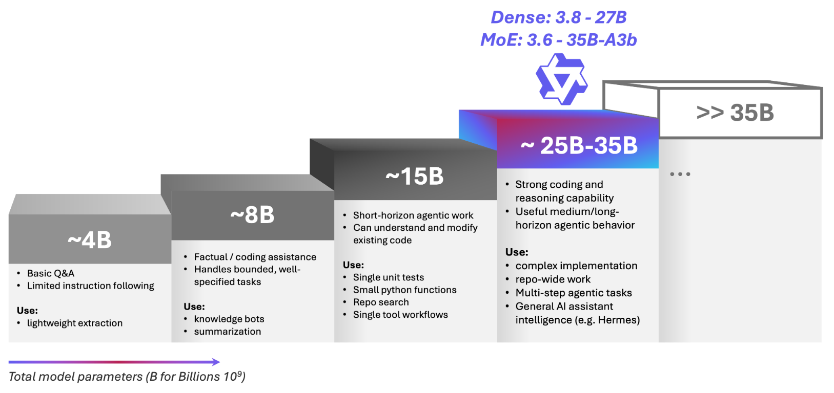
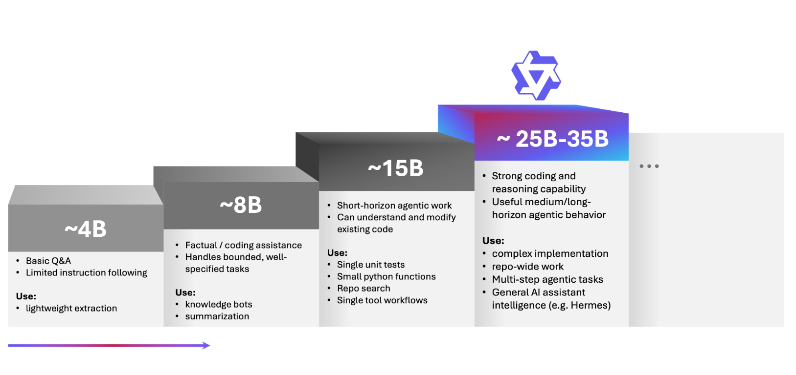
For my work (coding, agentic engineering), that sweet spot is the 25–35 billion parameter class. In practice that meant the dense Qwen 3.8 27B and the mixture-of-experts Qwen 3.6 35B-A3B. Note that the two numbers are not directly comparable: a mixture-of-experts model with 35 billion total parameters only activates about 3 billion of them per token, so it is much faster than a dense 27B model but behaves differently on harder tasks. Relating this back to the inference setup, the Splash engine in LM Studio on the Mac gives me about 77 tokens per second of generation with Qwen 3.8 27B, with a 3.2-second time to first token. With Qwen 3.6 35B-A3B it gives me about 244 tokens per second, with a 0.6-second time to first token. Both numbers come from the same prompt of roughly 3,500 input tokens and about 960 output tokens, with a 120K context window.
This is a statement about my hardware and my work, not a general ranking. With more memory, the sweet spot moves up. With a different workload, it might move down. The local models I used most, and the builds I ran, are listed at the end of this post.
What the usage data shows
Because Copilot was exporting telemetry the whole time, I can compare the two periods directly. The explorer below uses a snapshot of that data through November 17, 2026, and opens on the comparison I find most telling: every prompt I typed, plotted by the size of its largest model call and by its trajectory score, for each period on identical logarithmic axes.
The vertical axis is the trajectory score: how much observable agent activity one prompt caused. A prompt is one request I typed, plus every model call and tool call the agent made to answer it. The score is a weighted complexity formula over the three components the telemetry can observe:
Each component is log-scaled and normalized by its 95th percentile across all prompts:
where stands for each of the three components:
- is the agent depth: the number of sequential agent iterations for , measured as the highest recorded turn index plus one. Very long runs only export their last turn event, so this is a lower bound.
- is the prompt position: the 1-based position of in its chat session, a proxy for how much conversation came before it.
- is the number of tool calls linked to , or 0 if none were observed.
The logarithm compresses large values: going from 1 to 5 tool calls counts far more than going from 20 to 25, so one very long run does not flatten everything else. Dividing by the 95th percentile, P95, puts the components on a common scale; otherwise prompt position would dominate simply because its numbers are larger. In this data the P95 values are 18 agent iterations, the 76th prompt in a session and 26 tool calls, so equal weights of one third mean equal influence. A prompt at P95 on all three components scores exactly 1. Because depth and position are at least 1, the lowest possible score is about 0.13: a single-step first prompt without tools. A mid-sized prompt, with 5 agent iterations, at position 10 and with 8 tool calls, scores about 0.61, and the highest score in this data is 1.56.
Each prompt is plotted once, at the input tokens of its largest model call and at ; plotting every call would turn a long agent run into a row of dozens of dots. Calls from Copilot's utility models, the small background models VS Code uses for tasks such as chat titles and commit messages, are drawn separately as diamonds, one per call: I did not choose them, so they do not decide where a prompt sits. During the local-only weeks those utility tasks also ran on my local models and were recorded as ordinary local calls, so the diamonds only appear in the hybrid panel. I left out the thinking-token and output-token terms from my talk: the telemetry does not record thinking tokens, and output tokens measure verbosity as much as work. A high score means more observed agent activity, not a harder or better task.
During the local-only weeks, a typical prompt's largest call was about 32,000 input tokens. In the hybrid period the picture splits. Local prompts dropped to a median of about 25,000 tokens. That drop is mostly the harness, not the work: I ran most local prompts through the lightweight PI harness instead of VS Code, whose system prompts take considerably more tokens. Cloud prompts moved right, to a median of about 82,000 tokens, and 267 of 697 reached 100,000 tokens or more, against only 6 of 553 local prompts. Per call the gap is similar: a median of about 92,000 input tokens for cloud against about 31,000 for local.
The explorer's routing view shows the rule behind that split. Below about 15,000 tokens almost no prompt went to the cloud, around 40,000 it was a coin flip, and above 100,000 tokens 97% or more did. The trajectory score rises with prompt size too, which is why the cloud triangles sit a little higher, but at the same size it says little about where a prompt went. What decided the route was how much context a task needed, not how many agent steps it took.
I did not plan that division. Once I could choose again, large-context work went to the cloud, and the steady stream of small and medium tasks stayed local. The explorer also has a daily view with my holidays shaded and a breakdown of prompt sizes, and its method note lists what is excluded. The data shows how I used the models, not how productive I was or how good the code turned out. And the harness is not the whole story behind those shrinking local prompts. Part of it is in how the cloud and local models ended up working together.
Where local helped, and where it struggled
Local models were good at more than I expected. Repo search and code understanding were reliable. Writing unit tests was a strong fit. So was spotting bugs, brainstorming possible solutions, and command-line work. Bounded implementation was the real surprise: when a larger frontier model had written a clear specification, a 27B local model implemented features from it well. It was also useful for less obvious jobs, such as turning PDFs into HTML versions we could use as templates, or brainstorming different ways to rewrite text for articles. On top of that, for any work too sensitive for cloud AI, it ensured I still had my trusty AI agents alongside me.
Once the hardware and runtime settings were tuned, performance was good enough that I stopped noticing it. Local inference also has two quieter benefits: predictable cost, and no dependency on whether a cloud service is available or rate-limited that afternoon.
Where it struggled was just as clear. Long refactors that touch many files drifted. Very large repositories pushed against context limits and slowed everything down. And questions that need broad, current knowledge read from many sources rather than reasoning alone, such as detailed Terraform questions about Azure, is what frontier models were simply better at. A smaller model can reason well about code in front of it; it cannot know what it was never trained on. Complex architecture questions were less reliable locally, and long, high-iteration agent runs still favored the frontier models.
And of course, getting there took significant tinkering. Performance depended heavily on the runtime, the quantization and the hardware configuration.
The workflow that stayed
When I turned cloud models back on, I did not simply go back to how I worked before. Over the following weeks a workflow settled in that uses each tier for what it is good at. It is a form of spec-driven development.
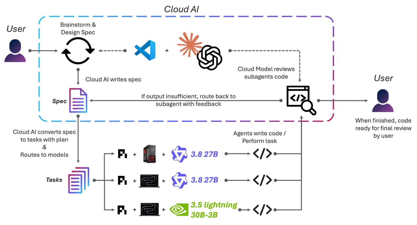
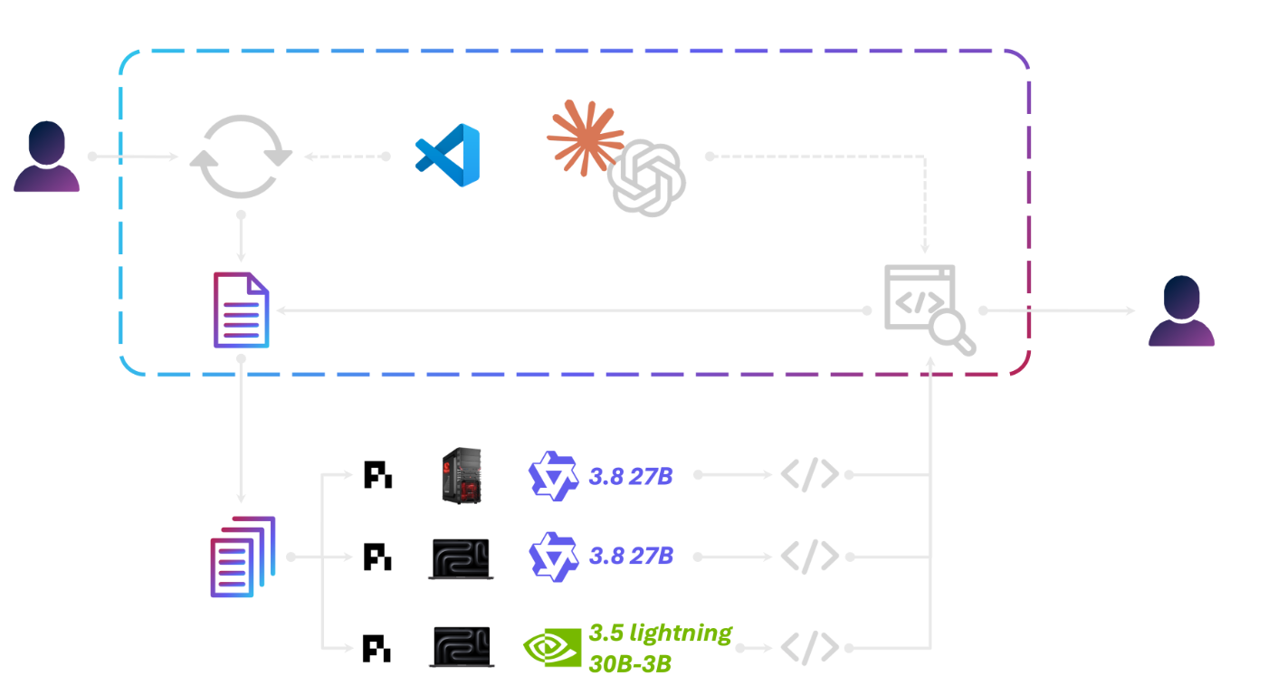
It starts with me, a cup of coffee and a frontier cloud model in VS Code, brainstorming and turning an idea into a written specification. Nothing moves until I approve that spec. The cloud model then breaks it into smaller tasks with a plan, and I approve that breakdown too, including which model runs each task. In my repos the cloud model keeps track of each local model's performance to help with estimating task sizes. Most implementation tasks go to local workers in their own isolated environments with clean contexts: Qwen 3.8 27B on the desktop or the MacBook, or an NVIDIA 30B mixture-of-experts model when speed matters more than depth. When a worker finishes, a cloud model reviews the result. If the output is not good enough, the task goes back to the worker with concrete feedback. When everything is done, the code comes to me for a final review.
The roles follow the data. The cloud tier does what needs long context, broad knowledge and careful judgment: design, planning and review. The local tier does the bulk of the bounded execution, where a capable 27B model is fast, predictable and essentially free to run. The tasks are small enough that context stays manageable, and the spec is clear enough that a local model does not need to guess. I later turned this workflow into a custom agent, which you can download at the end of this post.
Conclusion
So, could I replace my Ferrari with a bicycle? Unsurprisingly, I found out that we best use both. Local AI did not replace cloud AI; it became a complementary compute tier. Local models can cover a meaningful share of professional coding work, especially bounded implementation, repo exploration, code understanding and medium-complexity tasks. The strongest setup is hybrid: local models for capable, cost-effective execution, and frontier models for long context, deep reasoning, orchestration and final review. And running local AI means running AI infrastructure. The best results require tuning models, runtimes, memory, quantization, context and hardware. It is not a plug-and-play replacement for the cloud, but with some care it is a very good partner to it.
If you want to try this setup yourself, the orchestrator agent and the local models I used most are below.
The agent behind the workflow
The PI Harness Spec Orchestrator is a custom agent for VS Code Copilot that encodes the workflow described above. It turns a request into an approved specification and small tasks, asks me to choose the exact model for each PI worker, dispatches the work, has the result reviewed, and only closes a task after I approve it. The orchestrator itself is model-agnostic. The split between cloud and local in the diagram above is how I use it, not something hardcoded.
Three small skills handle the mechanics. The first runs each PI worker in a visible, persistent Terminal session, so I can watch what it does and step in when needed. The second records the handoffs, progress and recovery checkpoints for each task in the repository, so work survives a restart. The third handles a worker that stops making progress: it checks the evidence and asks me how to recover, instead of silently retrying.
Download the PI Harness Spec Orchestrator (v9) and its three skills. The bundle contains the orchestrator agent, the running-visible-pi-subagents, tracing-agent-orchestration, and handling-subagent-stalls skills, and a README with setup requirements (VS Code Copilot, PI, tmux, macOS Terminal). Configure model IDs for your own environment before use. Licensed under Apache 2.0.
The local models I used most
The three most-used local base models in the measured data, July 9 to November 17, 2026. Builds of one base model are counted together; estimated calls are left out.
| Base model | Calls | Share of 6,009 | Variants used |
|---|---|---|---|
| Qwen3.8 27B | 3,440 | 57.2% | LM Studio Splash; Unsloth UD-Q4_K_XL GGUF; oQ4; MTPLX Speed; NVFP4; 4-bit |
| Qwen3.6 35B-A3B | 1,179 | 19.6% | Qwen release in LM Studio; MLX 4-bit; Splash |
| Qwen3.6 27B | 830 | 13.8% | Qwen release; MTPLX Quality and Speed; MLX 4-bit; ThinkingCap fine-tune |
- The telemetry is a mix of four sources: Copilot in VS Code, Copilot agents and CLI, Codex, and the PI harness. Local calls from October 5 onward were not recorded, so the explorer estimates them. From August 3 to October 3 I made about one local call per cloud call (4,554 local, 4,512 cloud). Each later day gets that ratio, varied by a random day factor, times its cloud calls, minus the local calls that were recorded. No day exceeds my busiest recorded local day in September (919 calls), holidays get no estimate, and prompt sizes are drawn from the reference period. These 6,898 estimated calls count as local in the call counts and prompt sizes, but have no trajectory score. ↩